
티스토리 뷰
0. 분류의 성능 평가 지표
- 정확도(Accuracy)
- 오차행렬(Confusion Matrix)
- 정밀도(Precision)
- 재현율(Recall)
- F1 스코어
- ROC AUC
1. 오차행렬(confusion matrix)
- describe the performance of a classification model
- 학습된 분류 모델이 예측을 수행하면서 얼마나 헷갈리고 있는지 함께 보여주는 지표
- 이진 분류의 예측 오류가 얼마인지와 더불어 어떠한 유형의 예측 오류가 발생하고 있는지를 함께 나타내는 지표
- TN : 예측값을 Negative 값으로 0으로 예측했고 실제값 역시 Negative 값 0
- FP : 예측값을 Positivie 값 1로 예측했는데 실제값은 Negative 값 0
- FN : 예측값을 Negative 값 0으로 예측했는데 실제값은 Positive 값 1
- TP : 예측값을 Positive 값 1로 예측했는데 실제 값 역시 Positive 값 1
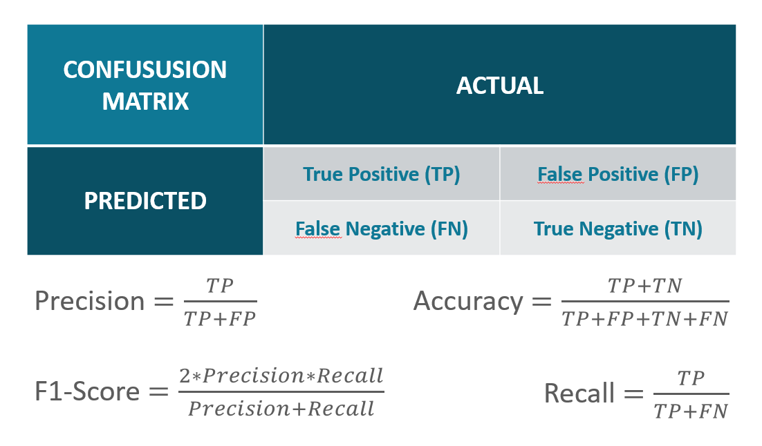
1.1 정확도(Accuracy)
- 실제 데이터에서 예측 데이터가 얼마나 같은지 판단
1.2 정밀도 (Precision)
- 예측을 Positive로 한 대상 중에 예측과 실제 값이 Positive로 일치한 데이터의 비율
- 정밀도가 중요 지표인 경우? 실제 Negative인 일반메일을 Positive인 스팸메일로 분류할 경우 메일을 아예 받지 못하게 되어 업무에 차질이 생김
1.3 재현율(Recall)
- 실제값이 Positive인 대상 중에 예측과 실제 값이 Positive로 일치한 데이터의 비율
- 재현율이 중요 지표인 경우? 실제 Positive 양성 데이터를 Negative로 잘못 하게 되면 업무상 큰 영향 생기는 경우
- ex) Positive 암환자를 Negative로 판단하면 엄청난 문제 발생
1.4 F1 - Score
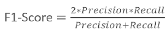
- 정밀도와 재현율을 결합한 지표
- F1 스코어는 정밀도와 재현율이 어느 한쪽으로 치우치지 않는 수치를 나타낼때 상대적으로 높은 값을 가짐
2. ROC 곡선과 AUC
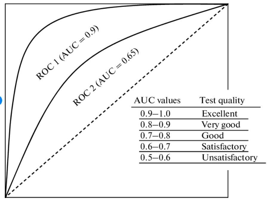
2.1 ROC 곡선(Receiver Operation Characteristic Curve)
- 우리말로는 수신자 판단 곡선
- 일반적으로 의학 분야에서 많이 사용되지만, 머신러닝의 이진 분류 모델의 예측 성능을 판단하는 지표
- ROC 곡선은 FPR(False Positive Rate)이 변할 때 TPR(True Positive RAte)이 어떻게 변하는지 나타내는 곡선
2.2 AUC(Area Under Curve)
- ROC 곡선 밑의 면적을 구한 것으로서 일반적으로 1에 가까울수록 좋은 수치
- AUC 수치가 커지려면 FRP이 작은 상태에서 얼마나 큰 TPR을 얻을 수 있느냐가 관건
3. python 코드
- Pima Indians Diabetes Database
- 데이터 셋 이용
|
1
2
3
4
5
6
7
8
9
10
11
12
13
14
15
16
17
18
19
20
21
22
23
24
25
26
27
28
29
30
31
32
33
34
35
36
37
38
39
40
41
42
43
44
45
46
47
48
49
50
51
52
53
54
55
56
57
58
59
60
61
62
63
64
65
66
67
68
69
70
71
72
73
74
75
76
77
78
79
80
81
|
import numpy as np
import pandas as pd
import matplotlib.pyplot as plt
from sklearn.model_selection import train_test_split
from sklearn.metrics import accuracy_score, precision_score, recall_score, roc_auc_score
from sklearn.metrics import f1_score, confusion_matrix, precision_recall_curve, roc_curve
from sklearn.preprocessing import StandardScaler
from sklearn.linear_model import LogisticRegression
from sklearn.metrics import roc_auc_score
def get_clf_eval(y_test,pred):
confusion = confusion_matrix(y_test,pred)
accuracy = accuracy_score(y_test,pred)
precision = precision_score(y_test,pred)
recall = recall_score(y_test,pred)
f1 = f1_score(y_test, pred)
roc_score = roc_auc_score(y_test,pred)
print("오차행렬")
print(confusion)
print('정확도 : {0:.4f}, 정밀도 : {1:.4f}, 재현율 : {2:.4f}, F1 : {3:.4f}, ROC AUC 값 {4:.4f}: '.format(accuracy, precision, recall, f1, roc_score))
diabets_data = pd.read_csv('diabetes.csv')
print(diabets_data['Outcome'].value_counts())
"""
0 500
1 268
"""
print(diabets_data.head(5))
"""
Name: Outcome, dtype: int64
Pregnancies Glucose BloodPressure ... DiabetesPedigreeFunction Age Outcome
0 6 148 72 ... 0.627 50 1
1 1 85 66 ... 0.351 31 0
2 8 183 64 ... 0.672 32 1
3 1 89 66 ... 0.167 21 0
4 0 137 40 ... 2.288 33 1
"""
print(diabets_data.info())
"""
[5 rows x 9 columns]
<class 'pandas.core.frame.DataFrame'>
RangeIndex: 768 entries, 0 to 767
Data columns (total 9 columns):
Pregnancies 768 non-null int64
Glucose 768 non-null int64
BloodPressure 768 non-null int64
SkinThickness 768 non-null int64
Insulin 768 non-null int64
BMI 768 non-null float64
DiabetesPedigreeFunction 768 non-null float64
Age 768 non-null int64
Outcome 768 non-null int64
"""
X = diabets_data.iloc[:,:-1]
y = diabets_data.iloc[:,-1]
X_train, X_test, y_train, y_test = train_test_split(X,y,test_size = 0.2, random_state = 156, stratify =y)
lr_clf = LogisticRegression()
lr_clf.fit(X_train,y_train)
pred = lr_clf.predict(X_test)
get_clf_eval(y_test,pred)
"""
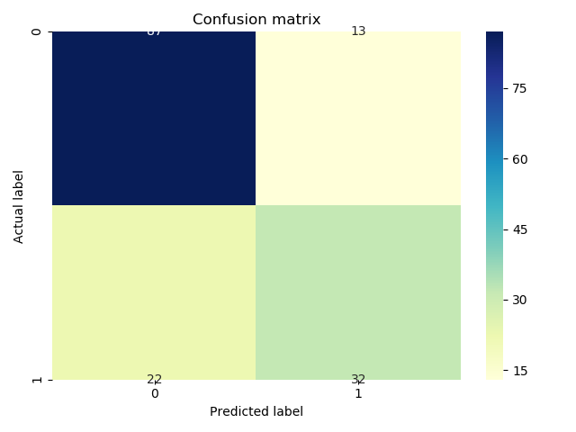
오차행렬
[[87 13]
[22 32]]
정확도 : 0.7727, 정밀도 : 0.7111, 재현율 : 0.5926, F1 : 0.6465, ROC AUC 값 0.7313:
"""
|
cs |
4. 오차 행렬(confusion matrix) - 숫자로 나타내기
|
1
2
3
4
5
6
7
8
9
10
11
12
|
from sklearn.metrics import confusion_matrix
confusion_matrix(y_test,pred)
result = pd.crosstab(y_test, pred, rownames=['True'], colnames=['Predicted'], margins=True)
print(result)
"""
Predicted 0 1 All
True
0 87 13 100
1 22 32 54
All 109 45 154
"""
|
cs |
5. 오차행렬(confusion matrix) - seaborn 으로 나타내기
|
1
2
3
4
5
6
7
8
9
|
from sklearn import metrics
import seaborn as sns
matrix = metrics.confusion_matrix(y_test,pred)
sns.heatmap(pd.DataFrame(matrix), annot=True, cmap="YlGnBu" ,fmt='g')
plt.title('Confusion matrix', y=1.1)
plt.ylabel('Actual label')
plt.xlabel('Predicted label')
plt.show()
|
cs |
<출처>
1. cubalytictalks.blogspot.com
DataScience by Cubalytics
Classication Task blog series
cubalytictalks.blogspot.com
2. roc curve 출처
3. data school
'인공지능 > 머신러닝' 카테고리의 다른 글
| 머신러닝 - 배치학습 vs 온라인학습 (0) | 2019.10.27 |
|---|---|
| Anaconda 기본 (0) | 2019.10.27 |
| [Math] 오일러 공식 Euler's Equation (0) | 2019.10.16 |
| [Math] 수학이야기 - Eigenvalue와 Eigenvector가 왜 중요할까 (0) | 2019.10.16 |
| 머신러닝 알고리즘 - 기저함수(basis function) (0) | 2019.10.16 |
댓글